ECON6037 Experimental Economics
Decision Under Risk
February 27, 2024
Introduction
In this lecture we will illustrate the concept of measurment using as an example measurement of risk aversion
Introduce the concept of choice under risk
Define measures of risk aversion
Construct behavioural measures
Discuss the relationship between behavioural measures and survey measures
Decision under risk
In many economic situations, decisions are made under risky or uncertain conditions
Utility framework under certainty to be extended to account for decision under risk or uncertainty
What are plausible requirements for this?
In many cases the outcome is money, so we restrict the view over utility over money. This is not innocuous as has been shown, as money does not give utility when one receives it.
Concept of Human Behaviour
Prototypical economists conception of human behaviour
\[ \max{x_i^t\in X_i}\sum_{t=0}^{\infty}\delta^t\sum_{s_t\in S_t}p(s_t)U(x_i^t|s_t) \]
- \(t\) time
- \(\delta\) time discounting
- \(x\) element of choice set (X)
- \(s\) element of possible states of the world (S)
- \(p(\cdot)\) belief over probability of a state occurring
- \(U(\cdot)\) utility depending on choice contingent on state
Rationality
What does it take for \(p(s_t)\) to be rational beliefs?
Having subjective probabilities that obey law of probability
- Probability that an event is happening lies between 0 and 1
- Probability that something happens is 1
- If events are disjoint their joint set is has the probability of the sum of the Individual probabilities
- Obey Bayes’ rule
Motivational Example
Motivational story by Savage (1954)
A businessman contemplates buying a certain piece of property. He considers the outcome of the next presidential election relevant. So, to clarify the matter to himself, he asks whether he would buy if he knew that the Democratic candidate were going to win, and decides that he would. Similarly, he considers whether he would buy if he knew that the Republican candidate were going to win, and again finds that he would. Seeing that he would buy in either event, he decides that he should buy, even though he does not know which event obtains, or will obtain, as we would ordinarily say. It is all too seldom that a decision can be arrived at on the basis of this principle, but except possibly for the assumption of simple ordering, I know of no other extra-logical principle governing decisions that finds such ready acceptance.
Sure thing principle
If \(\alpha \succ \beta\) if you knew that \(E\) occurred, and same if you knew that NOT \(E\) occurred, then you should \(\alpha \succ \beta\) regardless.
- Sure-thing makes utility independent across states
- Probability makes utility weights constant across acts
Probability and Sure principle imply expected utility theory, so we can write:
\[ U(x)=\sum_{s \in S} u(x,s)=\sum_{s\in S} u(x) p(s) \]
Preference over lotteries
Preferences over lotteries (q,r,s) can be represented by a utility function with the EU form \[EU= \sum_{\in I} p_i U(q_i)\] Preferences satisfy
- [Completeness] \(q > r\) or \(q = r\) or \(q < r\) for all \(q,r\)
- [Transitivity] \(q > r\); \(r > s\) \(\rightarrow\) \(q > s\)
- [Continuity] \(q > r\); \(r > s\); \(q > s\); Exist a \(p\) such that \(pq+(1-p)s = r\)
- [Independence of irrelevant alternatives] \(q > r\) \(\rightarrow\) \(q \dot p + s \dot (1-p)] > r \dot p + s \dot (1-p)\)
Relationship between utility function and risk aversion
Relates the value of a convex function of a sum (integral) to the sum (integral) of the convex function
If \(w\) is a random variable \(U(w)\) is
- [convex] \(\rightarrow EU (w) > U(E(w))\)
- [linear] \(\rightarrow EU (w) = U(E(w))\)
- [concave] \(\rightarrow EU (w) < U(E(w))\)
Measures of Risk Aversion
Given that the curvature of the utility function one can think of coarser measures of risk aversion
{Arrow–Pratt measure of absolute risk-aversion (ARA)}
\[ A(x)=-\frac{u''(x)}{u'(x)} \]
{Arrow-Pratt-De Finetti measure of relative risk-aversion (RRA)}
\[ R(x)=xA(x)=-\frac{x\cdot u''(x)}{u'(x)} \]
Functional forms
CARA
In the case of CARA, ARA must be constant
\[ A(x)=-\frac{u''(x)}{u'(x)} = cons. \]
one can show that this leads to a utility fuction of the following form:
\[ u(x) = -e^{-\theta x} \]
CRRA
In the case of CRRA, RRA must be constant
\[ R(x)=xA(x)=-\frac{x\cdot u''(x)}{u'(x)} = cons. \]
one can show that this leads to a utility fuction of the following form:
\[ u(x)= \begin{cases} \frac{1}{1-\theta}x^{1-\theta} & \mathsf{ if } \quad \theta>0 \mathsf{\quad and\quad } \theta \neq 1 \\ \ln x & \mathsf{ if } \quad \theta =1 \end{cases} \]
Elicitation Procedures Overview
- Different ways to elicit the risk attitudes
- The underlined attribute changes during the elicitation process
| Standard-gamble methods | |
|---|---|
| 1. Preference comparison | \(x_{1p} x_2 \text{ versus } x_c\) |
| 2. Probability equivalence | \(x_{1} \underline{p} x_2 \sim x_c\) |
| 3. Value equivalence | \(\underline{x}_{1p} x_2 \sim x_c\) |
| 4. Certainty equivalence | \(x_{1p} x_2 \sim \underline{x_c}\) |
| Paired-gamble methods | |
| 5. Preference comparison | \(x_{1p} x_2 \text{ versus } x'_{1p} x'_2\) |
| 6. Probability equivalence | \(x_{1\underline{p}} x_2 \sim x'_1p x'_2\) |
| 7. Value equivalence | \(\underline{x}*{1p} x_2* \sim x'{1p} x'_2\) |
Elicitation Procedures II
[Standard Gamble] Compare sure amount with non-degenerate lottery
[Paired Gamble] Compare two non-degenerate lotteries
[Probability equivalence] Elicit that makes subject indifferent
[Certainty equivalence] Elicit that makes subject indifferent
Under EU both methods are equivalent
Elicitation Procedures III
- Matching: Directly ask for the indifference point*{8pt}
- Bisection: convergent series of choices*{8pt}
- Bracketing: elicits indifference through series of choices*{8pt}
Elicitation Procedures IV
{Direct question} What amount of money, Eur , if paid to you with certainty, would make you indifferent to the lottery paying Eur ,(x_1) with probability (p) and Eur ,(x_2) with probability (1 - p).
- elicitation
- Dominated by choice based procedures
- They fead to fewer inconsistencies and less noise
Elicitation Procedures V
- : risky lottery vs riskless outcome
- For each iteration, the lottery chosen in bold.
- Depending on choice: certain outcome increased or decreased.
- Size of change half the size of previous change
- Leads to interval for the indifference value
- Midpoint taken as indifference value.
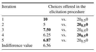
Bisection procedure
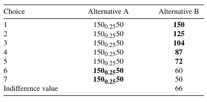
Bracketing procedure
- Standard gamble: risky lottery vs riskless outcome
- Seven choices in total
- Certain amounts are linearly spaced on the log scale
- Lottery chosen printed in bold
- Leads to interval for the indifference value
- Interval is taken as the indifference value
Bracketing procedure
Bracketing procedure
- Bracketing procedure is not chained: each choice is independent of previous choice
- For a given number of choices, bracketing is less precise
Trade-off precision and chaining}
if error propagation is an issue, bracketing should be preferred
if precision is a concern, bisection should be chosen
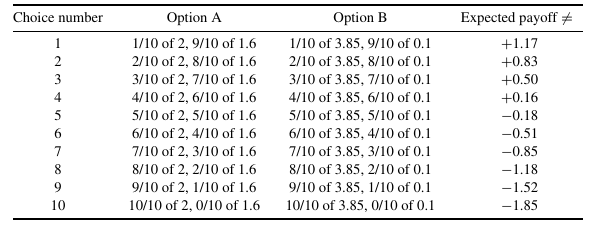
Bracketing procedure
- Ten different choices ordered by increasing probability (p) from (0.1) to (1)
- expected payoff difference between options (A) and (B),
- only extreme risk seekers choose B at any
- only extreme risk-averse DM keeps choosing option A for any probability (p) less
- no one should choose the dominated option A when the probability (p) is 1
frame
\[ p[(x_{A1} - x_{A2}) - (x_{B1} - x_{B2})] + (x_{A2} - x_{B2} ) \]
falls with (p) and is negative for \[ p > (x_{A2} - x_{B2} )/[(x_{B1} - x_{B2}) (x_{A1} - x_{A2} )] \]
risk-neutral individual switches from option A to option B when \[ p > (x_{A2} - x_{B2} )/[(x_{B1} - x_{B2} ) - (x_{A1} - x_{A2} )] \]. Switch point reveals risk attitude.
The Table shows the choices that the subjects face when (x_{A1} = 2), (x_{A2} = 1.6), (x_{B1} = 3.85 )and (x_{B2} = 5). %Subjects who switch from A to B between choices 4 and 5 are risk-neutral, while those %who switch between choices 2 and 3 are significantly risk-seeking and those switching %between choices 7 and 10 are significantly risk-averse.
Eliciting indifferences
Strength of eliciting indifferences allows direct estimation of individual relative risk aversion based on a particular utility function. Consider, constant relative risk-aversion (CRRA) utility function,
\[ u(x) = \begin{cases} x^{1-\theta}/(1-\theta) & \text{\, if\, } \theta \neq 1 \\ log(x) & \text{\, if\, } \theta = 1 \end{cases} \]
Shape of individual utility can be inferred from subject’s choices
How to get at parameter
EU maximiser with risk-aversion parameter \(\theta\) indifferent if \(\ldots\)
\[ p \times 21- \theta + (1 - p) \times 1.6 1-\theta = p \times 3.851-\theta + (1 - p) \times 51-\theta \]
Solving for \(\theta\) yields degree of risk aversion as a function of the probability \(p\) at which a subject switches between options A and B.
Paired Lottery Choice
- Switching point produces direct measure of CRRA index interval
- Subject switching between choices 4 and 5 close to risk-neutral
Precision: Not clear, where the subject’s preference lies in this interval: the subject may be slightly risk-averse, slightly risk-seeking or risk neutral.
Paired Lottery Choice
Paried Lottery Choice
Choose one of
| Choice (50/50 Gamble) | Low payoff | High payoff | Expected return | Standard deviation | Implied CRRA range |
|---|---|---|---|---|---|
| Gamble 1 | 28 | 28 | 28 | 0 | \(3.46 < r\) |
| Gamble 2 | 24 | 36 | 30 | 6 | \(1.16 < r < 3.46\) |
| Gamble 3 | 20 | 44 | 32 | 12 | \(0.71 < r < 1.16\) |
| Gamble 4 | 16 | 52 | 34 | 18 | \(0.50 < r < 0.71\) |
| Gamble 5 | 12 | 60 | 36 | 24 | \(0 < r < 0.50\) |
| Gamble 6 | 2 | 70 | 36 | 34 | \(r < 0\) |
Summarising the paired lottery choice
- Iterative
- Over Small and Large Stakes
- Data drives the functional form
- Can easily be extended to allow for Prospect Theory
- Utility between elicited points?
- Error correction?
Risk aversion in survey measures
German Socio Economic Panel (GSOEP)
Please tell me, in general, how willing or unwilling you are to take risks. Please use a scale from 0 to 10, where 0 means you are ”completely unwilling to take risks” and a 10 means you are ”very willing to take risks”. You can also use any numbers between 0 and 10 to indicate where you fall on the scale, like 0, 1, 2, 3, 4, 5, 6, 7, 8, 9, 10.
Dohmen et al., 2011 find a correlation coefficient between multiple price list method and question: \(0.4079\)
Experiment Overview and Risk Attitudes
- Contexts of Risk Attitudes: Examined in various domains like driving, finance, sports, work, health, and trust.
- Experiment Design:
- Conducted with 450 subjects, representative of the adult German population.
- Two-part approach: a questionnaire including a risk-related question, followed by a real-stakes lottery experiment.
- Lottery Experiment Details:
- 20 choices between a sure option and a lottery, with sure options ranging from 0 to 190 euros.
- The point where subjects switch from the lottery to the sure option indicates their risk aversion level.
Findings and Correlations
- Risk Attitudes Measurement:
- Median response to risk question: 5, Mean: 4.42, showing diverse risk attitudes.
- 78% exhibited risk aversion through their certainty equivalent.
- Correlation Between Survey and Real-Stakes Decisions:
- Significant correlation found between survey responses and choices in the lottery experiment.
- Consistency observed across different methods of risk attitude elicitation, with correlations ranging from 0.03 to 0.30.
- Principal-Components Analysis:
- Suggests a single behavioural trait underpins risk attitudes, with one component explaining 60% of variance in attitudes.
- International Findings:
- Similar findings across nearly 3,000 subjects in over 30 countries, showing a consistent pattern between incentivised measures and survey responses. (Vieider et al 2015)
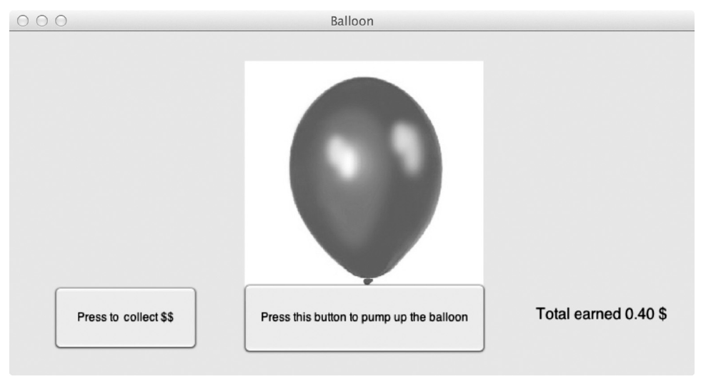
The balloon analogue risk task (BART)
(Lejuez et al., 2002)
Intuitive task to measure risk preferences without the usual numerical representation of lotteries
- The Task: Inflate a balloon by pumping air into it to earn money.
- Each pump inflates the balloon further and increases potential earnings.
- Participants have the option to “cash out” their earnings at any time.
- Risk of Explosion:
- If the balloon explodes, all earnings are lost.
- The challenge is to balance between earning more and the risk of explosion.
- Decision Making:
- Participants must decide when it’s best to stop pumping and secure their earnings.
- Sampling Mechanism:
- The process is akin to sampling without replacement from an unknown urn, where each pump represents a draw that could lead to an explosion or higher earnings.
BART picture
Bracketing procedure
BART correlates
- BART correlates with Holt Laury and survey question
- in BART, subjects show substantial risk lovingness while in other procedure subjects are more risk averse
- stopping point is not observed when the balloon
Structural estimation of Risk Aversion
Structural Decision Model
- structural decision model of choice by maximum likelihood
- (Z_j) dummy option (A) selected in choice (j)
- (U(A_j)) and (U(B_j)) value associated with prospects
- deterministic decision rule for EU maximiser \(DR_j = U(A_j) - U(B_j)\)
- DM chooses (A) over (B) in choice (j) if (DR_j > 0)
- (B) over (A) if (DR_j < 0), and is indifferent between them if (DR_j = 0)
frame
Decision rule parametrised by CRRA preference parameter ()
\(DR_j(\theta) = U(A_j|\theta)-U(B_j|\theta)\) predicts choices of A and B
Individuals make decision error ()
DM chooses \(A_j\) over option \(B_j\) if \(DR_j(\theta)+\epsilon_j > 0\)
Contradicts deterministic decision rule, if error large enough
frame
- where () is the error parameter.
- Noise parameter tends to 0 choice becomes deterministic
- Noise parameter tends to 1 choice becomes more random and